GIRAFFE [Kor]

Niemeyer et al. / GIRAFFE] Representing Scenes as Compositional Generative Neural Feature Fields / CVPR 2021 (oral, best paper award)

English version of this article is available.

1. Problem definition

GAN(Generative Adversarial Network) 을 통해 우리는 사실적인 이미지를 무작위로 생성할 수 있게 되었고, 더 나아가 각각의 표현(머리색, 이목구비 등)을 독립적으로 조절할 수 있는 경지에 이르렀다. 하지만 3차원 세계를 2D 로 나타냄으로써 한계에 부딪히게 되었고, 최근 연구들은 3D representation 을 효과적으로 나타내는 것에 주력하고 있다. 가장 대표적인 방법은 2장에서 소개될 implicit neural representation 인데, 지금까지의 연구들은 물체가 하나이거나 복잡하지 않은 이미지에 대해서만 좋은 성능을 보였다. 본 논문은 각각의 물체를 3D representation 의 개별적인 구성 요소로 대하는 생성 모델을 제안하여 여러 물체가 있는 복잡한 이미지에서도 좋은 성능을 보인다.

2. Motivation

Related work

Implicit Neural Representation (INR)

기존 인공신경망(neural network) 은 추정(ex. image classification) 과 생성(ex. generative models) 의 역할을 수행하였다. 이에 반해 Implicit representation 은 표현의 기능을 수행하여, network parameter 자체가 이미지 정보를 의미하게 된다. 그래서 네트워크의 크기는 정보의 복잡도에 비례하게 된다 (단순한 원보다 벌의 사진을 나타내는 모델이 더 복잡하다). 더 나아가 NeRF 에서 처럼 좌표가 입력값으로 들어왔을 때 RGB 값을 산출하는 연속적인 함수를 학습함으로써 연속적인 표현도 가능하게 되었다.

• NeRF : Neural Radiance Field $f_{\theta}:R^{L_x}\times R^{L_d}\to R^+ \times R^3$ $(\gamma(x),\gamma(d)) \to (\sigma, c)$

  하나의 장면은 5D 좌표 (3d 위치와 방향) 에 대한 RGB 값과 부피 intensity 을 산출하는 fully connected layer 로 표현된다. 이때 더 높은 차원의 정보를 얻기 위해 5D 입력값은 positional encoding $\gamma(x)$ 을 거치게 된다. 특정 방향에서 빛을 쏘았을 때 생기는 camera ray 내의 점을 n 개 샘플링한 후, 각각의 color 와 density 값을 volume rendering technique (3장 Methods 에 설명) 을 통해 합침으로써 이미지 pixel 의 값을 예측한다. 학습은 GT(ground truth) posed 이미지와 예측된 volume rendered 이미지 간의 차이를 줄이는 방향으로 이루어진다.

Figure 1: NeRF architecture

• GRAF : Generative Radiance Field $f_{\theta}:R^{L_x}\times R^{L_d}\times R^{M_s}\times R^{M_a} \to R^+\times R^3$ $(\gamma(x),\gamma(d),z_s,z_a) \to (\sigma, c)$

  본 논문은 NeRF 와 달리 unposed image 를 활용하여 3D representation 을 학습한다. Input 으로는 sampling 된 camera pose ε (위쪽 반구에서 중심을 바라보는 방향 중에서 uniform 하게 sample) 과 sampling 된 K x K patch (unposed image 에서 중심이 (u,v) 이고 scale 이 s 인 K x K 이미지) 를 가진다. 추가로, shape $z_s$ 와 appearance $z_a$ 코드를 condition 으로 넣어주어, patch 의 pixel 값을 예측하고, discriminator 에서 predicted patch 는 fake, 이미지 분포에서 sampling 된 image 의 실제 K x K patch 는 real 로 분류하는 학습을 진행한다.

Figure 2: GRAF architecture

Idea

GRAF 가 제어가능한 고해상도의 image synthesis 를 해내지만, 단일 물체만 있는 비교적 간단한 imagery 에서만 좋은 성능을 보이는 한계점을 가진다. 이를 해결하기 위해서, GIRAFFE 에서는 개별 object 를 구분하여 변형하고 회전시킬 수 있는 neural representation 을 제안한다.

3. Method

Figure 3: GIRAFFE architecture

• Neural Feature Field : GRAF formulation 과 유사하지만, 3D color 를 output 하는 것이 아니라 $M_f$-dimensional feature 를 output 한다. $h_{\theta}:R^{L_x} \times R^{L_d} \times R^{M_s} \times R^{M_a} \to R^+ \times R^{M_f}$ Object Representation NeRF 와 GRAF 에서는 전체 scene 이 하나의 model 로 표현 되었는데, 각 물체를 독립적으로 다루기 위해서 개별적인 feature field 로 나타낼 것을 본 논문에서는 제안한다. 이때 affine transformation도 parameter 를 dataset 에 의존적인 분포 활용함으로써 $T=\{s,t,R\}$ ($s$:scale, $t$: translation, $R$: rotation) 에서 샘플링함으로써 pose, shape, appearance 를 모두 제어할 수 있게 된다. $k(x)=R\cdot\begin{bmatrix} s_1 & & \\ & s_2 &\\ & & s_3 \end{bmatrix}\cdot x + t$ 그리고 나서 이산적으로 샘플링된 3D 데이터를 2D에 매핑하는 volume rendering 을 아래 식과 같이 진행한다. $(\sigma,f)=h_{\theta}(\gamma(k^{-1}(x)),\gamma(k^{-1}(d)),z_s,z_a)$ Composition Operator 각 scene 은 N 가지의 entitiy 로 정의된다(N-1 objects, 1 background). 각 entity 의 density 와 feature 를 합치기 위해 density-weighted mean 을 사용한다.

  $C(x,d)=(\sigma,{1\over\sigma} \sum_{i=1}^{N}\sigma_if_i), \quad where \quad \sigma = \sum_{i=1}^N\sigma_i$

  3D volume rendering 기존 연구들은 RGB value를 volume render 하는 반면, 본 논문은 $M_f$-dimensional feature vector $f$ 를 rendering 한다. 특정 camera ray $d$ 를 따라 샘플링된 $N_s$ 개의 포인트를 $\pi_{vol}$ operator 를 통해 최종 feature vector $f$ 를 얻는다. $\pi_{vol} : (R^+ \times R^{M_f})^{N_s} \to R^{M_f}$ 그 후 NeRF 와 동일하게 numerical integration 을 해준다. $f=\sum_{j=1}^{N_s}\tau_i\alpha_i f_i \quad \tau_j=\prod_{k=1}^{j-1}(1-\alpha_k) \quad \alpha_j=1-e^{-\sigma_j\delta_j}$ 위의 식에서 $\delta_j=|| x_{j+1} - x_j ||_2$ 는 주변 샘플 포인트와의 거리를 의미하고, 밀도값 $\sigma_j$ 와 함께 알파값 $\alpha_j$ 를 정의한다. 이 알파값들을 누적하여 투과도 $\tau_j$ 를 정의하고, 최종 feature vector $f$ 는 각 픽셀에 대해서 $\pi_{vol}$ 을 계산함으로써 얻어진다. 계산 효율성을 위해 피쳐 맵을 $16^2$ 크기로 얻는데, 이는 실제 이미지의 해상도인 $64^2$ 나 $256^2$ 에 못 미친다.

• 2D neural rendering 그래서 더 높은 해상도로 upsampling 하기 위해 아래 그림과 같은 방법으로 2D neural rendering 을 진행한다.

  $\pi_\theta^{neural}:R^{H_v \times W_v \times M_f} \to R^{H \times W \times 3}$

Figure 4: 2d neural rendering architecture

• Training

  • Generator

  $G_\theta(\left\{z_s^i,z_a^i,T_i\right\}_{i=1}^N,\epsilon)=\pi_\theta^{neural}(I_v),\quad where \quad I_v=\{\pi_{vol}(\{C(x_{jk},d_k)\}_{j=1}^{N_s})\}_{k=1}^{H_v \times W_v}$

  • Discriminator : CNN with leaky ReLU

  • Loss Function = non-saturating GAN loss + R1-regularization $V(\theta,\phi)=E_{z_s^i,z_a^i \sim N, \epsilon \sim p_T} [f(D_\phi(G_\theta(\{z_s^i,z_a^i,T_i\}_i,\epsilon))] + E_{I\sim p_D}[f(-D_\phi(I))- \lambda \vert\vert \bigtriangledown D_\phi (I) \vert\vert^2 ]$$\quad , where \quad f(t)=-log(1+exp(-t)), \quad \lambda=10$

4. Experiment & Result

Experimental setup

• DataSet

  • single object dataset로 자주 사용되는 Chairs, Cats, CelebA, CelebA-HQ

  • single-object dataset 중 까다롭다고 알려진 CompCars, LSUN Churches, FFHQ

  • multi-object scenes으로는 Clevr-N, Clevr-2345

• Baseline

  • voxel-based PlatonicGAN, BlockGAN, HoloGAN

  • radiance field-based GRAF

• Training setup

  • 한 장면 내의 entity 수 $N \sim p_N$, latent codes $z_s^i,z_a^i \sim N(0,I)$

  • camera pose $\epsilon \sim p_{\epsilon}$, transformations $T_i \sim p_T$ ⇒ $p_{\epsilon}$ 과 $p_T$ 는 uniform distribution 를 따른다고 가정하고 실험을 진행한다 (데이터 종속적인 camera elavation 과 object transformation)

  • 개별 object field 는 모두 MLP weight 를 공유하며 ReLU activation 을 사용한다.(object 들은 8 layers MLP(hidden dimension of 128), $M_f=128$ 를 사용하고, background 는 이의 절반을 사용한다.)

  • $L_x=2,3,10$과 $L_d=2,3,4$ 를 positional encoding parameter

  • 각 ray 따라 64 points를 sample 하고 image 별로 $16^2$ pixels 를 사용하여 계산 효율성을 얻는다.

• Evaluation Metric

  • 20,000 real & fake samples 로 Frechet Inception Distance (FID) score 계산

Result

• disentangled scene generation : background 와의 분리, feature 간의 분리 모두 잘 이루어진다

Figure 5: disentanglement

• comparison to baseline methods

Figure 6: qualitative comparison

• ablation studies

  • importance of 2D neural rendering and its individual components

    GRAF 와의 가장 큰 차이는 neural rendering 을 volumne rendering 과 함께 사용했다는 점이다. 이 방법은 모델의 표현력을 향상시키고 더 복잡한 real scene 도 다룰 수 있게 한다. 더 나아가, rendering 시간도 기존 GRAF 모델과 비교했을 때, $64^2$ pixels 이미지에서는 110.1ms 에서 4.8ms 로 줄었고, $256^2$ pixels 에서는 1595.0ms 에서 5.9ms 로 줄었다.

  • positional encoding

    $r(t,L) = (sin(2^0t\pi), cos(2^0t\pi),...,sin(2^Lt\pi),cos(2^Lt\pi))$

    

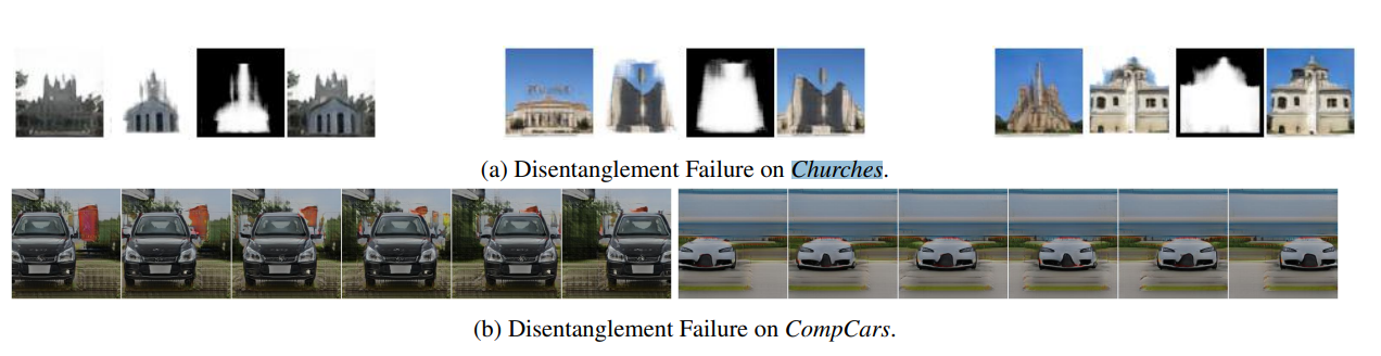
• limitations

  • 데이터 내에 inherent bias 가 있으면 같이 변화해야하는 factor 들이 고정되는 문제가 발생한다. (ex. 눈과 헤어 rotation)

  • camera pose 와 obejct 단위의 transformation 이 uniform distribution 을 따른다고 가정하는데, 실제로는 그렇지 않을 것이기에 아래와 같은 disentanglement failure 가 발생한다.

  

5. Conclusion

⇒ 한 장면을 compositional generative neural feature field 로 나타냄으로써, 개별 object 를 background 뿐만 아니라 shape 과 appenarance 로부터 disentangle 하였고, 별다른 supervision 없이 이를 독립적으로 control 할 수 있다.

⇒ Future work

• 개별 object 의 tranformation 과 camera pose 의 distribution 을 데이터로부터 학습할 수는 없을까?

• object mask 와 같이 얻기 쉬운 supervision 을 활용하면 더 복잡한 multi-object scene 을 더 나타낼 수 있을 것으로 보인다.

Take home message (오늘의 교훈)

• Implicit Neural Representation 을 활용한 3D scene representation 은 최근에 각광 받고 잇는 방식이다.

• 각각의 entity 를 개별 feature field 로 나타내는 것은 그들의 movement 를 disentangle 하는데 도움이 된다.

• 각 feature 를 원래 dimension 그대로로 사용하기 보다는 positional encoding 이나 neural rendering 을 통해 더 high dimensional space 로 embedding 하여 활용하면 더 풍부한 정보를 활용할 수 있게 된다.

Author / Reviewer information

Author

김소희(Sohee Kim)

• KAIST AI

• Contact: [e-mail]

Reviewer

1. Korean name (English name): Affiliation / Contact information

2. Korean name (English name): Affiliation / Contact information

3. ...

Reference & Additional materials

1. GIRAFFE paper

2. GIRAFFE supplementary material

3. GIRAFFE - Github

4. INR explanation

5. NeRF paper

6. GRAF paper